“Autonomous” means “self-governing”. In these equations, the rate of change of \(y\) depends only on \(y\) itself, not on time \(t\text{.}\) The system’s behavior is determined entirely by its current state. Think of a spring: it pushes back the same way no matter the time of day. Only how far it’s compressed matters, not what time it is.
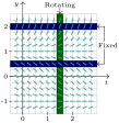
Here, the slope at any point \((t,y)\) depends only on \(y\text{.}\) Moving up or down (changing \(y\)) changes the slope, but sliding left or right (changing \(t\)) does not. The result is a “striped” slope field—each horizontal line has the same slope pattern all the way across.
Figure 85(a) illustrates this. As you go up the plane, the slope segments gradually rotate, reflecting how \(f(y)\) changes with \(y\text{.}\) But moving sideways leaves the segments fixed—the slopes don’t shift with \(t\text{.}\)
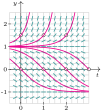
This symmetry isn’t just in the slope field; it shows up in the solutions themselves. As seen in Figure 85(b), if you know one solution curve for an autonomous equation, you can create others simply by shifting that solution horizontally. That’s because the equation doesn’t “know” what time it is; it only cares about \(y\text{.}\)
Suppose you compute the slope of an autonomous differential equation to be \(3\) at the point \((2, 1)\text{.}\) What is the slope at \((-3, 1)\text{?}\)